


There are two main reasons to consider analytics systems when dealing with evolving information in real time and near real time. One reason...
There are two main reasons to consider analytics systems when dealing with evolving information in real time and near real time. One reason is to sense and respond. In these situations, we want to monitor data to get a sense of what is happening in order to respond to it in a timely fashion. A second reason is to implement an early warning system. This includes timely collection and analysis of data, resulting in prompt interventions. We look at examples of both of these scenarios in the following sections. We also describe the concept of stream computing and describe a specific analytics system that we built using the principles of stream computing to harness the analytics from real-time and near real-time systems.
 While on the surface, this system seems like an interesting ruse to keep the attention of viewers, it is really validating an individual’s opinion with that of others. But what if this kind of technology could actually sway voters or public opinion one way or another? That’s exactly what British psychologists, Colin Davis, Amina Memon, and Jeffrey Bowers, of the Royal Holloway University of London believed.
In a simple experiment, Davis and his team had two groups of subjects watch an election debate that included the worm as an indication of others’ (supposedly undecided voters’) opinions. To test their hypothesis that the worm could influence public opinion, Davis and his team presented their subjects not true public opinion but fake data that would show the supposed opinion in favor of one candidate over the other.
Their results were intriguing, to say the least [3]. What they found was that the worm did have a huge influence on their subjects’ perception of who won the debate. The two groups had completely different ideas about who had won the debate, and their opinions were consistent with what the worm had been telling them (which, again, was manipulated by Davis and his team). So the group that saw a worm which favored Gordon Brown thought that he had won the debate, whereas the group that saw the worm which favored Nick Clegg overwhelmingly thought that he was the winner. Interestingly, when the research team asked their subjects about their choice of preferred prime minister, it was clear that, if people had been voting immediately after that debate, the manipulation could have had a significant effect on how those people voted!
We highlight this example to showcase the power of real-time analytics. If public opinion can be swayed by the opinions of others, it only stands to reason that from a business perspective, we would be served to understand the pulse of our constituents and look to re-emphasize the positive and correct the negative as soon as possible.
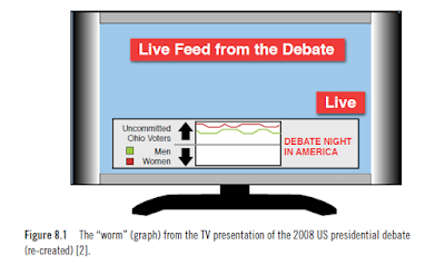
In the example in Figure 8.1, the sample audience members had a specialized device that allowed them to change their “feelings” about a candidate using a simple dial or switch. This data was polled and the results sent back to a central station to be aggregated and quickly displayed on national television. This type of scenario is pretty close to real time since there is no additional processing to take place, and the “signal,” or opinion, is fed right to the source (in this case, CNN).
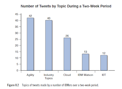
Because the data comes to us (or anybody) in essentially a random fashion, real time doesn’t make sense, so we aggregate it over a five-minute interval so that changes in the data are more apparent. For example, Figure 8.2 shows the top distribution of topics of conversation from Twitter made by a select group of IBMers. This data represents the topics as they were discussed at the time of the sampling, which was delayed by five minutes. Because the number of participants was low, the chance of the graph changing appreciably in real time was low, so we simply show it in near real time.

Think of a stream like a conveyor belt that delivers packets of information, or data, in a continuous flow (see Figure 8.4). This doesn’t mean the time between entries is consistent, but it does mean that data will continue to flow over time. As an item reaches the end of the belt (in our case, a system that can process data in motion), the item is processed, and then room is made to process the item on the belt in a sequential fashion.

This analogy works well from a data-arrival perspective. But what makes stream computing sometimes difficult to grasp is that the concept of querying the data is turned around somewhat. If we wanted to capture and analyze data in a traditional environment, we would set up a feed to capture all of the data we are interested in first and then analyze it. This process involves capturing data, storing it into some kind of a database, creating queries to run against the data, and then executing those queries and deriving some information.
With a stream model, we define the queries or manipulation process of the data first using something like IBM’s Streams Processing Language (SPL). We connect these nodes together in a directed graph (or a path for the data to flow through our system), and then rather than collect and query, we run the data over our graph and produce results as the data arrives.
Functions that operate on stream data are known as filters. Filters operate on stream data and then pass it along in the stream, continuing the flow, which results in another stream. A string of filters operating together is called a pipeline. Filters may operate on one item of a stream at a time or may base an item of output on multiple items of input from other parts of the stream. So, while we show a single stream in Figure 8.5, any number of streams of data may pass through an environment, combining items, separating items, and forming new streams along the way.

Stream computing can enable an organization to detect trends or signals in fast-moving data that can be detected or acted upon only at the time it occurs. With stream computing, we are able to process and potentially take action on rapidly arriving data because we are watching a data flow in its original sequence (in real time or near real time). As a result, we are able to analyze and act on issues before they are lost to history, or rather, before that needle gets lost in the haystack. As a result, there is now a paradigm shift as we move our processing data in batch (or operating on “data at rest”) to processing data in real time, thus enabling faster insights.
■ Processing elements (PEs)—A processing element is an individual execution program that performs some function on the incoming stream. Processing elements are then tied together to create a workflow of execution.
■ Tuples—An individual piece of information in a stream is called a tuple. This is essentially the piece of data that is passed along the stream from one processing element to the next. This data can be structured or unstructured. Typically, the data in a tuple represents the state of an object at a specific point in time—for example, the running sentiment of a Twitter feed, the current topics of conversation, or the reading from external sensors.
■ Data streams—These are the running sequence of data (in the form of tuples) that passes from one processing element to the next.
■ Operators—An SPL operator manipulates tuple data from the incoming stream and produces results in the form of an output stream. One or more operators work together to form multiple streams and operators deployed in streams to form a data flow graph.
■ Jobs—A job is an instance of a running streams processing application.
■ Ports—A port is the place where a stream connects to an operator. Many operators have one input port and one output port, but operators can also have zero input ports (for example, if we read from an external source), zero output ports (if an operator is performing an operation and storing the results in a database as opposed to passing tuple down the stream), or multiple input or output ports.
The tuple is the only data construct in streams. The data flow (streams) between the operators (processing elements) is made up entirely of tuples. We can say that the streams of a tuple are processed or manipulated to obtain the desired result. A tuple can have any number of elements (strings, numbers, and so on) within the construct and may even consist of another tuple. For the sake of simplicity, think of a stream as the data path and the contents of the stream being made up of tuples that get passed from one operator to the next (producing a new tuple to be passed on to the next operator).

The graph in Figure 8.6 is taken from our Simple Social Metrics application described later. Here, Operator1 has received some information from the Internet. Because we don’t require many of the fields that come in a standard feed from Twitter, our operator takes the raw data and creates a shorter subset of each tweet, Tuple1, and passes that data down the stream to Operator2. It is important to understand that these processing elements, or operators, are purposely meant to be simple in function. This provides for an environment that is then easy to modify by simply rearranging the order that the operators are located in the stream.
Operator2 in our application is a processing element that accepts two inputs: Tuple1 (the shortened form of the tweet from the Twitter stream) and another tuple, indicated by the solid triangle, that is the result of another operator. While we don’t show it in this diagram, the operator’s function is to take the tweet from the Twitter stream and perform a lookup in a table that we maintain. This list of special users is simply a list of known IBM tweeters, and if one of them has a tweet in the stream, we create a new tuple that contains not only that user’s tweet and Twitter handle, but also an indication of the fact that he or she is indeed an IBM employee. This way, we can segment or separate IBM opinion or comments from our customers if the need arises. The function of Operator2 is to merge that data, if necessary, and perform a sentiment analysis of the comment. The resulting data is represented as Tuple2 and then passed along the stream to the next operator.
In Operator3, the incoming data is categorized based on a simple dictionary lookup of terms. This allows us to group similar discussion topics together. Again, the data stream is modified and passed on to the next node in the stream as a new tuple (represented by the dark square). This is the beauty of streams. By turning as many functions into atomic or single-purpose functions as possible, we can quickly assemble a computational flow based on the type of analysis we are looking to perform.
While we plan to show a simple example of how we use Streams to capture this data in near real time, our system is a bit more complex in practice. We show a few of the metrics we derive, but since this is a discussion about possibilities as opposed to a how-to guide, we chose to show a subset. In our live system, we are able to derive the following attributes (in real and near real time) within a stream of Twitter data:
■ Top authors
■ Top hashtags
■ Top mentions
■ Top negative sentiments
■ Top positive sentiments
■ Top known tweeters based on a predetermined list
■ Top unknown tweeters based on a predetermined list
■ Top retweeted users
■ Top tweeted languages
■ Top words
■ Sentiment distribution (sentiment trend)
■ Sentiment count
■ Top reach (computed by author tweets multiplied by number
of followers)
■ Top categories
■ Author information with top-used negative and positive sentiment, top categories
■ Count trend over given period for tweets, hashtags, and mentions
For the purposes of this example, we discuss only top classifications, mentions, authors, and words. We have chosen only these four to illustrate the concept because they are some of the most commonly used metrics that we have encountered in our work. All of these metrics can be utilized to provide
business value depending on the project at hand.
Figure 8.7 shows an example of our near real-time engine for analyzing Twitter streams. We labeled each of the distinct steps 1 through 8.
 Let’s look at the flow of data in a step-by-step fashion, using the following
sample tweet: @mattganis loving working with #streams!
1. The first contains just the text of the tweet, also referred to as tweet payload. We use an external classifier in the next operator, but all we need for that is the text of the tweet itself.
2. In JSONtoTuple, we examine the tweet payload and look for any Twitter mentions in the stream. We want to keep track of who is being talked about in the Twitter stream, so we form a tuple that contains all of the @userid phrases that we encounter in the tweet.
3. We form a tuple that contains just the author of the tweet. This information is passed on to a separate operator that processes it alone (in this case, simply updating the author count in the database).
4. We create a tuple that contains all of the words used in the Tweet. That data is passed on to the next operator, and a word count is written to the database. This allows us to easily form word clouds based on the frequency of words used.
One of the outputs of the JSONtoTuple operator is the tuple we call tweet. It’s a stream representation of the tweet payload we just received (in this example, @mattganis loving working with #streams!). At this point, it’s placed in a stream that will take it to a classifier, so we can group similar tweets together. This same tuple is also sent (on another stream) at step 7, where it is broken down into the individual words for later use in a word cloud.
Step 4
We’ve found it useful to look at a large number of tweets and group them into “buckets,” or classifications, based on their subject matter. Classification is a difficult problem, but we take advantage of the fact that Twitter (or any microblogging technology) uses short text for updates coupled with the fact that when we gather Twitter data, we are gathering it based on a predetermined set of filters. In the case of the tweet used as an example for this section, #streams will probably translate into a category called “Stream Computing”. To explore this concept some more, let’s consider a few other examples. For example, in the past we have captured all of the tweets that contain the word #ibminterconnect, so more than likely any mention of the word cloud in a tweet that also has #ibminterconnect is probably talking about cloud computing technologies.
We chose to implement our classifier as a Web Service so that it can be utilized by a variety of applications. It doesn’t strive for perfection but gets pretty close. As we said earlier, we take advantage of the facts that tweets are generally short and we know the general theme of the topics. Our classifier is a simple pattern-matching algorithm based on categories and words that represent that category or indicate they are not part of that categorization.
For example:
Topic: Cloud Computing
Matches: cloud, Softlayer, PAAS, SAAS, Bluemix
Excludes: rain, snow, sleet, storm
Topic: Mobile
Matches: ipad, ipod, iphone, android, smart phone
Excludes: music, playlists, store
So if our classifier “sees” a tweet that contains the word bluemix, for example, we could return a classification of “Cloud Computing.” Of course, if the tweet contains any of the words from the exclude list, we don’t classify it as “Cloud Computing” and move on to the next category to be analyzed.
Tweets could discuss a variety of topics, and at times they overlap. So a tweet like the following would return two classifications (“Mobile” and “Cloud Computing”) because they have keywords that match both classifications:
@mattganis building a new iphone app on bluemix is easy!
database to be aggregated with other classifications.

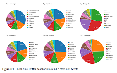
In the end, our real-time monitor looks something like Figure 8.9. During analysis, if we discover that some categories contain such a large number of tweets that the pie chart is dominated by that category, we are hardly able to get valuable information out of the rest of the categories. For example, in the bottom right of Figure 8.9, the pie chart shows the distribution of tweets based on the language. If English were included, we would not get any readable information about other languages. In cases like these, we record the value of tweets in the English language and then remove or deselect that category to convey more information. As a result, we are able to see the distribution of other languages such as Portuguese and Swedish.
Consider a keynote address that needs to be delivered to a large professional conference (or any other large presentation). Consider how much more effective a presentation could be if the speaker refers to topics that he or she knows are of interest to the audience. Sounds obvious, right? But we all know that, as human beings, our priorities, interests, and concerns are always in flux. Even the projects we work on are often moving targets. So how do we prepare to present a topic to an audience and address the topics currently on our (collective) minds ?
One way to do this is to monitor social media analytics strategy around the event and look for common themes or topics. Figure 8.10 shows some data from a recent trade show where we monitored the topics of conversation over time.
 Most conferences today use a Twitter hashtag to promote their event to allow participants to post comments or observations. So imagine you’re about to deliver an address to this large crowd. In the morning, the hot topic of conversation at the conference was security (with over 40% of the tweets discussing some aspect of the topic), followed by cloud computing with 26% of the discussion. But by mid-afternoon, the topic of conversation has changed (somewhat drastically) to indicate that almost half of the conversation is centered around the topic of cloud computing (at 48%) with the second topic shifting from security to the Internet of Things (IoT). With this information in hand, you can shift the emphasis of your talk from security to cloud computing given that it is still relevant to your original topic. So if your plan was to focus on security (or even mobile applications), it’s clear (at least from a social media data mining discussion) that these topics may not be the uppermost in your audience’s minds. A slight tweak to your presentation to highlight areas around the Internet of Things focusing on cloud technologies would, it appears, be much more appealing.
Another application of this technique could be in the context of panel discussions, talk shows, or any live event. If, indeed, you monitor the conversation in social media and aggregate the results (as we did in the previous example), questions to panelists or topics of discussion become much more relevant (and useful) to those listening, thereby increasing the value of your participation. One key point to remember is that you need to understand your audience and determine if what is happening in socia l venues is truly a representation of their views.
Is There Value in Real Time?
During the 2008 US presidential debates, a TV channel used a real-time public opinion display (see Figure 8.1) to depict the averaged reactions of 32 supposedly undecided voters. They expressed favor or disfavor for the candidates by turning handheld dials as they watched the debates live. The results of those public opinions were immediately converted into a real-time computer-generated graph. This graphic, also referred to as the worm, was displayed at the bottom of millions of television screens to give an indication of the public’s approval or disapproval of the comments the leaders were making. This could be considered an example of a sense-and-respond system. We are sensing in real time the opinions of a small group of individuals, and in response, we are translating that into a graphic that is being shared with millions of users.
In a simple experiment, Davis and his team had two groups of subjects watch an election debate that included the worm as an indication of others’ (supposedly undecided voters’) opinions. To test their hypothesis that the worm could influence public opinion, Davis and his team presented their subjects not true public opinion but fake data that would show the supposed opinion in favor of one candidate over the other.
Their results were intriguing, to say the least [3]. What they found was that the worm did have a huge influence on their subjects’ perception of who won the debate. The two groups had completely different ideas about who had won the debate, and their opinions were consistent with what the worm had been telling them (which, again, was manipulated by Davis and his team). So the group that saw a worm which favored Gordon Brown thought that he had won the debate, whereas the group that saw the worm which favored Nick Clegg overwhelmingly thought that he was the winner. Interestingly, when the research team asked their subjects about their choice of preferred prime minister, it was clear that, if people had been voting immediately after that debate, the manipulation could have had a significant effect on how those people voted!
We highlight this example to showcase the power of real-time analytics. If public opinion can be swayed by the opinions of others, it only stands to reason that from a business perspective, we would be served to understand the pulse of our constituents and look to re-emphasize the positive and correct the negative as soon as possible.
Real Time Versus Near Real Time
We draw a distinction between real time and what we like to call near real time. Think of real time as being instantaneous access to data: The second someone says or does something, we are notified right away. In the case of near real time, we assume there is some delay in between the time an event occurred and our notification or observance of the event. What makes it “near” real as opposed to analyzing prior data is that the time between the event’s occurrence and our observation is minimized. Basically, we acknowledge the fact that most of what we observe in real time isn’t instant, simply due to the processing or analysis that must be done to make sense of the event.In the example in Figure 8.1, the sample audience members had a specialized device that allowed them to change their “feelings” about a candidate using a simple dial or switch. This data was polled and the results sent back to a central station to be aggregated and quickly displayed on national television. This type of scenario is pretty close to real time since there is no additional processing to take place, and the “signal,” or opinion, is fed right to the source (in this case, CNN).
Because the data comes to us (or anybody) in essentially a random fashion, real time doesn’t make sense, so we aggregate it over a five-minute interval so that changes in the data are more apparent. For example, Figure 8.2 shows the top distribution of topics of conversation from Twitter made by a select group of IBMers. This data represents the topics as they were discussed at the time of the sampling, which was delayed by five minutes. Because the number of participants was low, the chance of the graph changing appreciably in real time was low, so we simply show it in near real time.

Forewarned Is Forearmed
So why look at data in real time? What value is there? Consider the case of IBM’s Always-On Engagement Center. Figure 8.3 shows an example of a display often used by IBM Engagement Center at various IBM events around the world . The idea behind the display is to highlight, in real time, analyze social media data conversations happening at that moment around a given topic. While some insightful bits of information emerge, the Engagement Center allows a user, at a moment’s notice, to gauge the pulse of a community or the thoughts or feelings around a topic. Using these techniques, command centers or call centers can, in theory, be ready for an onslaught of calls pertaining to a particular issue or incidence. So again, while not providing an insight into why something happened, we can be prepared for it by understanding what the discussion is around a particular topic. This can be considered an example of an early warning system.
Stream Computing
Stream computing is one of the latest trends allowing organizations to continuously integrate and analyze data in motion in an effort to deliver real-time and near real-time analytics. For the purposes of computing analytics, a stream is nothing more than a sequence of data elements delivered for processing over a continuous time frame.Think of a stream like a conveyor belt that delivers packets of information, or data, in a continuous flow (see Figure 8.4). This doesn’t mean the time between entries is consistent, but it does mean that data will continue to flow over time. As an item reaches the end of the belt (in our case, a system that can process data in motion), the item is processed, and then room is made to process the item on the belt in a sequential fashion.

This analogy works well from a data-arrival perspective. But what makes stream computing sometimes difficult to grasp is that the concept of querying the data is turned around somewhat. If we wanted to capture and analyze data in a traditional environment, we would set up a feed to capture all of the data we are interested in first and then analyze it. This process involves capturing data, storing it into some kind of a database, creating queries to run against the data, and then executing those queries and deriving some information.
With a stream model, we define the queries or manipulation process of the data first using something like IBM’s Streams Processing Language (SPL). We connect these nodes together in a directed graph (or a path for the data to flow through our system), and then rather than collect and query, we run the data over our graph and produce results as the data arrives.
Functions that operate on stream data are known as filters. Filters operate on stream data and then pass it along in the stream, continuing the flow, which results in another stream. A string of filters operating together is called a pipeline. Filters may operate on one item of a stream at a time or may base an item of output on multiple items of input from other parts of the stream. So, while we show a single stream in Figure 8.5, any number of streams of data may pass through an environment, combining items, separating items, and forming new streams along the way.

Stream computing can enable an organization to detect trends or signals in fast-moving data that can be detected or acted upon only at the time it occurs. With stream computing, we are able to process and potentially take action on rapidly arriving data because we are watching a data flow in its original sequence (in real time or near real time). As a result, we are able to analyze and act on issues before they are lost to history, or rather, before that needle gets lost in the haystack. As a result, there is now a paradigm shift as we move our processing data in batch (or operating on “data at rest”) to processing data in real time, thus enabling faster insights.
IBM InfoSphere Streams
IBM InfoSphere Streams is a software platform that enables the development and execution of applications that process information in data streams. Streams enables continuous and fast analysis of massive volumes of moving data to help improve the speed of business insight and decision making. Streams consists of a programming language and an Integrated Development Environment (IDE) for Streams applications and a runtime system that can execute the applications on a single or distributed set of hosts. The Streams Studio IDE includes tools for authoring and creating visual representations of the Streams applications. Streams offers the IBM Streams Processing Language (SPL) interface for end users to operate on data streams. SPL provides a language and runtime framework to support streaming applications. Users can create applications without needing to understand the lower-level stream-specific operations. SPL provides numerous built-in operators, the ability to import data from outside streams and export results outside the system, and a facility to extend the underlying system with user-defined operators. Many of the SPL built-in operators provide powerful relational functions such as Join and Aggregate.SPL Applications
The main components of SPL applications are as follows:■ Processing elements (PEs)—A processing element is an individual execution program that performs some function on the incoming stream. Processing elements are then tied together to create a workflow of execution.
■ Tuples—An individual piece of information in a stream is called a tuple. This is essentially the piece of data that is passed along the stream from one processing element to the next. This data can be structured or unstructured. Typically, the data in a tuple represents the state of an object at a specific point in time—for example, the running sentiment of a Twitter feed, the current topics of conversation, or the reading from external sensors.
■ Data streams—These are the running sequence of data (in the form of tuples) that passes from one processing element to the next.
■ Operators—An SPL operator manipulates tuple data from the incoming stream and produces results in the form of an output stream. One or more operators work together to form multiple streams and operators deployed in streams to form a data flow graph.
■ Jobs—A job is an instance of a running streams processing application.
■ Ports—A port is the place where a stream connects to an operator. Many operators have one input port and one output port, but operators can also have zero input ports (for example, if we read from an external source), zero output ports (if an operator is performing an operation and storing the results in a database as opposed to passing tuple down the stream), or multiple input or output ports.
The tuple is the only data construct in streams. The data flow (streams) between the operators (processing elements) is made up entirely of tuples. We can say that the streams of a tuple are processed or manipulated to obtain the desired result. A tuple can have any number of elements (strings, numbers, and so on) within the construct and may even consist of another tuple. For the sake of simplicity, think of a stream as the data path and the contents of the stream being made up of tuples that get passed from one operator to the next (producing a new tuple to be passed on to the next operator).
Directed Graphs
A directed graph is a graph or set of objects (called vertices or nodes) that are connected together. When we think about streams, the nodes or vertices are essentially represented as processing elements (which are further composed of operators). These edges are directed from one vertex to another (passing tuples) along a data stream (see Figure 8.6).
The graph in Figure 8.6 is taken from our Simple Social Metrics application described later. Here, Operator1 has received some information from the Internet. Because we don’t require many of the fields that come in a standard feed from Twitter, our operator takes the raw data and creates a shorter subset of each tweet, Tuple1, and passes that data down the stream to Operator2. It is important to understand that these processing elements, or operators, are purposely meant to be simple in function. This provides for an environment that is then easy to modify by simply rearranging the order that the operators are located in the stream.
Operator2 in our application is a processing element that accepts two inputs: Tuple1 (the shortened form of the tweet from the Twitter stream) and another tuple, indicated by the solid triangle, that is the result of another operator. While we don’t show it in this diagram, the operator’s function is to take the tweet from the Twitter stream and perform a lookup in a table that we maintain. This list of special users is simply a list of known IBM tweeters, and if one of them has a tweet in the stream, we create a new tuple that contains not only that user’s tweet and Twitter handle, but also an indication of the fact that he or she is indeed an IBM employee. This way, we can segment or separate IBM opinion or comments from our customers if the need arises. The function of Operator2 is to merge that data, if necessary, and perform a sentiment analysis of the comment. The resulting data is represented as Tuple2 and then passed along the stream to the next operator.
In Operator3, the incoming data is categorized based on a simple dictionary lookup of terms. This allows us to group similar discussion topics together. Again, the data stream is modified and passed on to the next node in the stream as a new tuple (represented by the dark square). This is the beauty of streams. By turning as many functions into atomic or single-purpose functions as possible, we can quickly assemble a computational flow based on the type of analysis we are looking to perform.
Streams Example: SSM
As discussed before, we’ve created a simple but effective application based on InfoSphere Streams that we call Simple Social Metrics, or SSM. The idea behind this system is to capture a stream of tweets around a predetermined topic and provide summary analytics around the stream in real or near real time. Our system also supports an analysis of the stream in the past because we record our data to a standard SQL database, which in turn is front-ended by a number of REST Application Programming Interfaces (APIs) for querying the data. REpresentational State Transfer, or REST, is an architectural style and an approach to communications that is often used in the development of Web services. The use of REST is often preferred over the more heavyweight Simple Object Access Protocol (SOAP) style because REST does not leverage as much bandwidth, which makes it a better fit for use over the Internet.While we plan to show a simple example of how we use Streams to capture this data in near real time, our system is a bit more complex in practice. We show a few of the metrics we derive, but since this is a discussion about possibilities as opposed to a how-to guide, we chose to show a subset. In our live system, we are able to derive the following attributes (in real and near real time) within a stream of Twitter data:
■ Top authors
■ Top hashtags
■ Top mentions
■ Top negative sentiments
■ Top positive sentiments
■ Top known tweeters based on a predetermined list
■ Top unknown tweeters based on a predetermined list
■ Top retweeted users
■ Top tweeted languages
■ Top words
■ Sentiment distribution (sentiment trend)
■ Sentiment count
■ Top reach (computed by author tweets multiplied by number
of followers)
■ Top categories
■ Author information with top-used negative and positive sentiment, top categories
■ Count trend over given period for tweets, hashtags, and mentions
For the purposes of this example, we discuss only top classifications, mentions, authors, and words. We have chosen only these four to illustrate the concept because they are some of the most commonly used metrics that we have encountered in our work. All of these metrics can be utilized to provide
business value depending on the project at hand.
Figure 8.7 shows an example of our near real-time engine for analyzing Twitter streams. We labeled each of the distinct steps 1 through 8.

sample tweet: @mattganis loving working with #streams!
Step 1
Streams has a number of built-in functions that allow a programmer to ingest data from a variety of sources. In this case, we connect to the Twitter source and read the tweets that we have collected that were a match to our search criteria. In many examples, we set up a Twitter feed and simply watch for a hashtag or small number of keywords that, when matched, will be collected by our search engine for later retrieval and ingestion (like we do here). In this step, we start with an operator that receives a stream of tweets in the form of JSON data [5]. JavaScript Object Notation is a lightweight data-interchange format. It is easy for humans to read and write; plus, it is easy for machines to parse and generate. That data, in JSON format, is collected externally and read by our first operator (called ReadTweet). The data is separated by tweet (the input data source could be composed of a number of tweets) and formed into a tuple that is passed along the stream to the next operator (in this case, JSONtoTuple).Step 2
The JSONtoTuple operator has an input port (for the incoming tuple, which contains the tweet to be analyzed) and several output ports (each of which has a different tuple placed on it). Here, we form four different tuples:1. The first contains just the text of the tweet, also referred to as tweet payload. We use an external classifier in the next operator, but all we need for that is the text of the tweet itself.
2. In JSONtoTuple, we examine the tweet payload and look for any Twitter mentions in the stream. We want to keep track of who is being talked about in the Twitter stream, so we form a tuple that contains all of the @userid phrases that we encounter in the tweet.
3. We form a tuple that contains just the author of the tweet. This information is passed on to a separate operator that processes it alone (in this case, simply updating the author count in the database).
4. We create a tuple that contains all of the words used in the Tweet. That data is passed on to the next operator, and a word count is written to the database. This allows us to easily form word clouds based on the frequency of words used.
Step 3
It’s important to remember that steps 3, 5, 6, and 7 all execute at the same time (in parallel). So even though they are labeled numerically (to help us understand this example), the power of stream computing is that tasks can happen simultaneously.One of the outputs of the JSONtoTuple operator is the tuple we call tweet. It’s a stream representation of the tweet payload we just received (in this example, @mattganis loving working with #streams!). At this point, it’s placed in a stream that will take it to a classifier, so we can group similar tweets together. This same tuple is also sent (on another stream) at step 7, where it is broken down into the individual words for later use in a word cloud.
Step 4
We’ve found it useful to look at a large number of tweets and group them into “buckets,” or classifications, based on their subject matter. Classification is a difficult problem, but we take advantage of the fact that Twitter (or any microblogging technology) uses short text for updates coupled with the fact that when we gather Twitter data, we are gathering it based on a predetermined set of filters. In the case of the tweet used as an example for this section, #streams will probably translate into a category called “Stream Computing”. To explore this concept some more, let’s consider a few other examples. For example, in the past we have captured all of the tweets that contain the word #ibminterconnect, so more than likely any mention of the word cloud in a tweet that also has #ibminterconnect is probably talking about cloud computing technologies.
We chose to implement our classifier as a Web Service so that it can be utilized by a variety of applications. It doesn’t strive for perfection but gets pretty close. As we said earlier, we take advantage of the facts that tweets are generally short and we know the general theme of the topics. Our classifier is a simple pattern-matching algorithm based on categories and words that represent that category or indicate they are not part of that categorization.
For example:
Topic: Cloud Computing
Matches: cloud, Softlayer, PAAS, SAAS, Bluemix
Excludes: rain, snow, sleet, storm
Topic: Mobile
Matches: ipad, ipod, iphone, android, smart phone
Excludes: music, playlists, store
So if our classifier “sees” a tweet that contains the word bluemix, for example, we could return a classification of “Cloud Computing.” Of course, if the tweet contains any of the words from the exclude list, we don’t classify it as “Cloud Computing” and move on to the next category to be analyzed.
Tweets could discuss a variety of topics, and at times they overlap. So a tweet like the following would return two classifications (“Mobile” and “Cloud Computing”) because they have keywords that match both classifications:
@mattganis building a new iphone app on bluemix is easy!
So at step 4,
the tweet is formatted into a REST service call and sent out for a classification. When the results are returned, they are parsed and put into yet another tuple, which is then sent onto its next step in the stream. In that step, the operator writes the data on the tweets classification into thedatabase to be aggregated with other classifications.
Steps 5 and 6
We’ve grouped steps 5 and 6 together because they do essentially the same thing (but with different slices of the data). In step 5, the operator receives a tuple that was formed in the JSONtoTuple operator; it contains all of the Twitter handles that were mentioned in the tweet (anything with an @ symbol in front of it). Mentions are useful for determining who is being talked about or referred to in a given tweet (perhaps leading to an influencer). This list of Twitter handles is simply written to the database, so we can quickly determine how many mentions any given Twitter handle received over a given time period. In our example, we save the handle @mattganis in the database. Step 6 is similar; here, we receive a tuple that contains just the author of the tweet, which is immediately written out to our database. This step is useful for understanding who is conversing the most in a given stream of Twitter conversations.Steps 7 and 8
Step 7 is another workhorse operator. Here, the input to the operator is a tuple that contains the tweet payload (@mattganis loving working with #streams!). In this step, we parse the tweet and remove all common words (things like a, and, with, and so on) and just keep the relevant words. They are put into a tuple and passed on to step 8, where they are written to the database as well. What this allows us to do is query for the top words (and their frequency) in a stream and form a word cloud (such as the one shown in Figure 8.8), where the larger and darker a word, the more it was used, and the smaller and lighter, the less often it was used.
In the end, our real-time monitor looks something like Figure 8.9. During analysis, if we discover that some categories contain such a large number of tweets that the pie chart is dominated by that category, we are hardly able to get valuable information out of the rest of the categories. For example, in the bottom right of Figure 8.9, the pie chart shows the distribution of tweets based on the language. If English were included, we would not get any readable information about other languages. In cases like these, we record the value of tweets in the English language and then remove or deselect that category to convey more information. As a result, we are able to see the distribution of other languages such as Portuguese and Swedish.

Value Derived from a Conference Using Real-Time Analytics
Consider a keynote address that needs to be delivered to a large professional conference (or any other large presentation). Consider how much more effective a presentation could be if the speaker refers to topics that he or she knows are of interest to the audience. Sounds obvious, right? But we all know that, as human beings, our priorities, interests, and concerns are always in flux. Even the projects we work on are often moving targets. So how do we prepare to present a topic to an audience and address the topics currently on our (collective) minds ?
One way to do this is to monitor social media analytics strategy around the event and look for common themes or topics. Figure 8.10 shows some data from a recent trade show where we monitored the topics of conversation over time.

Another application of this technique could be in the context of panel discussions, talk shows, or any live event. If, indeed, you monitor the conversation in social media and aggregate the results (as we did in the previous example), questions to panelists or topics of discussion become much more relevant (and useful) to those listening, thereby increasing the value of your participation. One key point to remember is that you need to understand your audience and determine if what is happening in socia l venues is truly a representation of their views.


COMMENTS